
Paraguay is
located in central South America, surrounded by Bolivia, Argentina and Brazil,
within the latitude and longitude of
23°00´ S, 58°00´ W with a population is 6,000,000 people. The total land area of the
country is 406,750 sq km, with 31.1% of forest land area. The economy of the
country is based on agricultural production including cattle rising. The
primary sector represents almost 20% do the GNP (14 billion US$. In 2010), out of with forest production covers 6% (2010), with a decreasing
trend[2].
(See Table 1, 11 and 12 and Figure 1 in Annexe)
The
Forestry Law of Paraguay states in its Article 42 that all farms with more than
20 hectares of land must have at least 5% of the total area covered with forest
or tree plantation. For farms with forest cover, one fourth must be kept[3]. The application of the law was
highly limited by implementation and enforcement problems and up to certain
point due to lack of political interest. Consequently, between 1973 and 2000, Paraguay lost almost
two-third of its Atlantic Forest (Per. comm.. Monges, L. 2011).
In
2008, after 61 years in power the Colorado Party lost the presidential election
to a coalition lead by the Liberal party along with many small left-wing
oriented parties. The new authorities, many of them coming from the NGOs
sectors (very critical of the intensive farming system applied by agribusiness-operated commercial farm) started to
enforce the Forestry Law given a high priority to the Article 42.
The
Federation of Production Coops from Paraguay (FECOPROD)[4]
gathers most of the agriculture cooperatives in the country[5].
The majority of its members are coops with agribusiness-operated
commercial farm, specialized in annual crops production (soybean, maize
and wheat), beef for the local and external markets, and milk for the local
market. Due to the size of their farm they are also know as medium and large
size farmers[6].
FECOPROD
reacted to the enforcement of the law by preparing an appraisal of the Forestry
situation of its cooperatives members and by developing a strategic plan
(2011-2005) for the sector[7].
The title of the document “Forestry
Development: An option integrated to the agriculture production”[8]
shows the compromise or the aim of the Federation to support or encourage its
cooperatives members to include tree plantation into the farming system in
compliance with the Article 42 of the Forestry Law.
Farmers in
Paraguay in general have increased interest in tree plantation due to scarcity
of fuel wood and the constant price increase of commercial wood[9].
Farmers want to profit from this market opportunity, taking into consideration
the climate conditions in the country is excellent for growing trees. Currently, two coops associated to
FECOPROOD, Cooperativa Colonias Unidas y Cooperativs Volendam[10],
have already developed some schemes to support tree plantation. The former one
provides loans fuel-wood production to be used in the drying of grain. Salas
(2010) provides an excellent description on the use of fuelwood by Cooperativa
Colonias Unidas.
The
specialized literature, as so far reviewed, main focus in on agroforestry
systems for small peasant farmers or at a more aggregate level. Besides, some
studies done from Australian Government Authorities, there are few studies for
an agribusiness-operated commercial farm. For
a successful timber production within those farms, to
which this paper focuses, a scientific designed system is needed. The system
must include the complementary effects of tree planting into the net returns of
the farm. However, relatively little information exists on designing an optimal
tree plantation system combining both biophysical information and economic or
financial information for any type of farm in Paraguay.
The
limitation of data on the on the one hand causes that feasibility decisions must often be
made on incomplete or preliminary data. On the other hand imposes the need to
develop practical methods to address the complexity of financial and economic
evaluation of agroforestry systems. The methodology must take into account the
bio-physical implications of agroforestry. The identification of the
opportunity cost of different alternatives with methodologies that includes
bio-physical information will allow the correct or proper allocation of the
resources in the farm. The reality of Paraguay is that for agroforestry projects, there is often
little experimental quantification of possible complementary or supplementary
biological responses to intercropping.
In order to
assess the profitability of tree planting, the most common action is to use economic
analyses. The use of economic will help answer questions such as: (1) what is
the optimal combination of two options of agroforestry, known as joint
production possibility, (2) what is the best or optimal mix of options to apply
to a given area? (Thomas, 1991). In short, what it has to be assessed is the
cost of the forgone benefits of the farmer due to the plantation of trees in
his farm. This is known as the opportunity cost.
The
opportunity cost of different agroforestry possibilities can be measured from a
very wide set of options, starting at a very elemental and basic static
cost–benefit passing through dynamic modeling and econometric analyses which
requires the use of powerful software and statistical packages (Brown,
2000; Graves, 2007; Borner, J.
et al. 2009). As progress is made towards the last ones, the
quality of the data also increases and the level of details is more demanding.
In developing countries, the availability of data (economic as well as
bio-physical) limits the implementation of most modeling as well as econometric
analyses[11],
(Brown, 2000; Graves,
2007) not to mention limitations in the qualification of human resources.
The
political decision by the Federation been taken; now the efforts are
concentrated on developing the assessment methodology of introducing trees
plantation into agricultural farms.
At
this point some questions arise:
a)
It
is a fact that farmers want to make profit from their farming activities, so
how will tree plantation impact on the profitability of the farm in a scenario
characterized by high commodity prices and the forecast that they will keep
increasing? What is the opportunity cost?
b)
Another
fact is that there is almost no forest area left on most farms. Then, is 5% area
profitable or it will mean a reduction in the farm profits? What about larger
areas, let us say 7%, 15%, 20% or more? What is the break even area in relation
to the size of the farm?
c)
If
timber production is an option for diversification of farm income activities, as
frequently cited in the specialized literature, how should it combine with
annual crops in order to maximize benefits taking into account the production
factors endowment of the farm?
d)
The
usual feasibility studies of the cooperative to decide on loans are financial
in essence. Then what about the economic and environmental gains including
positive externalities?
e)
Assuming
that re-planting the obligated 5% trees does not have a positive return to the
farmer, should society, through taxes, provide subsidies to a
re-planting/re-forestation scheme or program?
f)
What
is the “model” to be implemented? In the specific case of interest of this paper
the idea of agroforestry is a little different of what is more commonly
understood[12]. The
interest of farmers is towards intercropping of pure tree plantation in one
plot and pure crop plot plantation, not a mixing of both in the same plot. An
explanation could be the fact that their labour is dependent on machines
(mechanized farms) rather than hand-working as peasant-farmers do. Then, what
is the combination of trees an crops, plant density, rotation period,
management system, etc.?
g)
What
technical coefficients for tree growing shall be used, knowing the shortage of
systematic research on the subject in the country?
II.
OBJECTIVE
The
overall objective is to develop a methodology to assess the feasibility
(financial, economic and environmental) of introducing tree plantation into the agribusiness-operated commercial
farms. It will answer the question of
whether silvoarable[13]
forestry could provide a profitable alternative land use in areas dominated by annual
commodities crops.
Due
to the broad scope of the overall objective, intermediate ones are set. The
first specific objective concentrates on financial aspects: to determine the
opportunity costs of the introduction of tree planting in the farm production
system. Agribusiness-operated
commercial farms main
objective is capital
accumulation and income generation. Any other benefits accrued from their
farming activities are considered as by-products. Then, the financial profitability of
reforestation investment will be a key issue for the development of private
plantation forestry.
Therefore,
the first step is to know the financial methodologies by which investments in
agro-forestry and tree plantation are evaluated. To avoid reinventing the
wheel, a literature review of the methods use in financial appraisal will be
implemented as well as the identification of the inputs needed to apply the
reviewed methods. Additionally, some examples found in the specialized
literature will be presented.
The review summarizes the key elements of the existing approaches to
evaluate the impact of tree planting in a farm. The following tools are reviewed: (a) Classical
project evaluation technique also known as cost-benefit analysis: (b) Linear
programming; (c) Bio-economic models. The review of each methodology is
organized as follows: (a) description of the tools, (b) The information needed;
(c) Examples of the application of the tool.
a) Cost-benefit analysis
Three
are the most common cost-benefit analysis indicators use to measure the financial
and economic performance of an agroforestry project: Net Present Value (NPV),
Internal Rate of Return (IRR) and Ratio Benefit/cost (B/C). The combined used
of three indicators for each option allows the identification of the best
alternative. Decision based only on of the indicators ignoring the analysis of
the ohters may lead to improper selection.
The steps for an assessment using these tools include (Betters, 1988; Thomas, 1991)
·
Identify
relevant inputs.
·
Quantify the
levels of inputs to be used according to technical coefficients related to the
local conditions.
·
Simulate the
production of the timber and the agricultural output.
·
Calculate cost,
revenues and cash flow of the alternatives being analyzed for the years of the
rotation
·
Calculate the
indicators: NPV, B/C and IRR.
·
Make
sensitivity analysis of price and discounted rates
·
Analyze the
information and select the alternative
The rate used for discounting has to represent the
opportunity cost of the farmer, meaning the best alternative to de current
activity. When the estimation of this rate may create some difficult, the
interest rate paid on loans to which the farmer have access to it is commonly
used as a proxy (Betters, 1988). When such information is not available, different
methodologies are applied. The formula of the net present value is (Betters,
1988):

Internal rate of return: It is the rate which the NPV equal zero,
meaning that higher rates will represent negatives NPV. Putting it in a
different context, the IRR represents the maximum return rate possible to the
investor or the maximum time preference rate for the farmer. The decision
follows this rule: if IRR is greater than the cost of the capital or the
minimum acceptable rate of return stated by the investor the project is
accepted. IRR, though commonly use in project appraisal, has a severe
limitation. It ignores the timing and relative magnitude of costs and returns. The
IRR formula is as follows (Betters, 1988).

Benefit-cost ratios: It is the ratio of discounted
benefits/discounted costs, representing the benefit for each unit of money
invested. The B–C ratio of greater than 1 indicates that the project is
profitable. It can be calculated with the following formula (Betters, 1988).

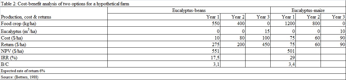
In Table 2
in Annexes, uses of the indicators are illustrated. Using a case extracted from
Betters, (1988), where the farmer has to decide introduce Eucalyptus in his
farm and has to choose between two options of agroforestry: Eucalyptus and beans and Eucalyptus and maize. The table shows
the production, the cost and the return for the investment for each of the
options. Since the time frame of the investment, all values are brought to the
first year using a discount rate of 6%. The rotation period is three years.
Let us
analyze the results: (Table 2, in Annexes)
The
Eucalyptus-beans option might be the elected one based on a greater NPV and an
IRR superior to the expected rate of return. However, in a situation where
access to loans is limited, the other option, Eucalyptus-maize would be chosen
for it has a greater return on every monetary unit invested. This is to say
that every 100 $ invested returns with a profit of 240 $, while in the other
option is 210 $. Beside, the return from Eucalyptus-maize is almost 13 points
above that of Eucalyptus-beans.
Prices can
decrease over the period of the agroforestry scheme, affecting farmers benefit
and specifically NPV, IRR and B/C. The same impact can cause an increase in the
interest rate. The possible impact is measured by means of a sensitivity
analysis, consisting in changing the price (reduction and increase) and their
impact on the assessment indicators. The usual analysis is conducted by
reducing selling prices and increasing discount rate. In Table 3 in Annexes an
increase in the discount rate reduces shows the effects on the NPV. In situations of uncertainty caused
by lack of adequate data on prices for instance, or difficulties to select a
proper discount rate, sensitivity analysis is a must in the assessment of
projects. Some examples on the use of benefit-cost analysis in farming decision
are presented in the Table 4.
b) Linear programming
Linear
programming (LP) is a mathematical model able to calculate the optimal
allocation of resources (land, capital and labour) between alternatives
(agroforestry or monocropping) that will maximizes the net present value of the
farm. At the same time, LP satisfies the specified constrains and requirements stated
by farmers. The optimum may include
either maximization (incomes for instance) or minimization (costs for instance)
(Verinumbe, Knispscheer and Enabor, 1985; Thomas, 1991; Bertomeu, Bertomeu and Gimenez
2006)
Basically, LP finds the solution by solving a series of linear equations.
Some basic problems can even be solved by hands, but the common practice is to
use softwares; LINDO Systems[14], GAMS[15],
XPRESS-MP[16].
Microsoft Excel has a complement called Solver which is a powerful optimization and resource
allocation too (Aieta, 1997).
To clarify
the functioning of linear programing, let us resource to an example developed
by Bertomeu, Bertomeu and Gimenez (2006)
In order to
“run” a LP exercise some information and data has to be collected. The first
group of data includes the resource availability (or constraints from another
point of view). In the example they are land, capital and labour. In this
specific case, the farmer adds two other constrains, as they are the
requirements of protein income and fuelwood demand are needed. The term “constrains”
is used in the sense that the selected solution must fulfill the required
constraints. For instance, the solution cannot demand more than 900 hours of
labour or produce less than 60 m3 of fuelwood. A second group of information is
related to technical coefficients and budget requirements. They are gross
margin and labour demanded per hectare. Finally, all the information is fed
into the program. See Table 5 in Annexes
The mains
results are organized in three groups. The first is the maximum possible gross
margin. The second group contains the area of cultivation of each one of the
alternative. Finally, there is information on the use of the resources o the
accomplishment of minimum requirements (fuelwood and protein). In the specific
case of Solver, it provides other information such as the opportunity cost of
each one of the restriction (constraints) and of how changes in the value of
the parameters affect the optimum solution (sensitivity analysis).
LP has some
limitation that must be taking into consideration. It is applicable only in
situations where the objective or constrains can be expressed as a straight
line equation. Furthermore, parameters used are assumed to constant. Reality is
not linear nor constant, at least not always. Linear programming models assigns
portions of the farm to the different options (monocropping, intercropping,
fallow, etc.). They do not provide information on the exact location and
arrangement of the options. To do so a spatially explicit programming model
need to be used (Mendoza, et al. 1986; Wojtkowski, Brister and Cubbage, 1988). .
Qualitative
or variable factors as weather conditions are not taken into consideration. It
does not consider (or does not quantifies) others benefits-ecological, social,
economical and cultural. In short, it ignores the multidimensionality of
agroforestry. One alternative is to use multi-objective programming for it can
optimize several objective functions simultaneously (Mendoza, et al. 1986;
Wojtkowski, Brister and Cubbage, 1988; Bertomeu, Bertomeu and Gimenez 2006). However,
as Bertomeu, Bertomeu and Gimenez (2006)) state, when it is assumed that the
main objective of the farmers is financial benefits (as it is most of the
time), LP is well suited.
Research using
LP was common in the 1980s. Some examples of the use of LP in farming decision
are presented in the Table 6 of Annexes.
c) Bio-economic models
The
development of computer science and the easy access to computers, favored the
investigation to more complex and elaborated tools for optimization and
modeling the reality. The
identification of the opportunity cost of different alternatives with
methodologies that includes bio-physical information will allow the correct or
proper allocation of the resources in the farm (Brown, 2000; Kruseman, 2000;
Stewart, H. et al. 2011).
Nowadays it
is common to use simulation models to measure recreate the effects of changes
in some of the variable of a system (Brown, 2000). These models can be applied at
the farm-house level or at the aggregate level (village, watershed, community
of users) or even for global simulations. Pure economic models run short of
describing the effect on production, farm profitability and environmental
impacts of the decision-making. Most suitable for these purposes are the
bio-economic models. They deal with the modeling of decision-making and the
modeling of biological processes (Ruben et al, 2000, cited by Brown, 2000). Bio-economics models are in the middle of the
spectrum economic-biophysical models. As stated by Graves et al (2007) they can
go from a “detailed biophysical model
with limited economic analysis to economic models that use biophysical data
from an external source”
An economic
model aims to model the decision making process of humans, while the biological
attempts to model the biological processes. For instance, a simple economic
model as LP optimizes farm incomes. However, it becomes a bio-economic model
when it includes biophysical features that attempts to measure biological or
ecological processes as well. To do so, it can use as proxy level of erosion, (Brown, 2000; Namaalwa, Sankhayan
and Hofstad 2007).
More
sophisticated models includes multiple objective programming for a variety of objective such as the maximization of financial returns, maximization of timber volume or number
of cows grazed, or maintenance of the site for ecological purposes (Mendoza et
al, 1986). They aim to simulate the dynamic relationships of biological and economic processes (Brown, 2000).
Biological
models are designed to simulate agro-ecological processes. They model plant and
animal growth, soil physical characteristics and nutrient flows and balances,
as well as interspecies interaction, competition and feedback from one subsystem
components to the other (Brown,
2000). The biological
models cover a great deal of agro-ecological processes: forestry, crop
production, grassland, savannah, soil nutrients, and water dynamics and animal/livestock
systems. Basic biological models uses empirical measures of biological
processes (Pulina et al, 1999; Kruseman, 2000) while others more sophisticated
attempt to model the underlying processes or mechanisms at a more basic level.
Ruben
et al, 2000 (cited by Brown, 2000) describes ideal bio-economic models as those
that
“… capture the dynamic nature of the
biological processes involved and allow for dynamic feedback effects between
human decisions, biological processes, and the range of possibilities available
for future decisions. An ideal bio-economic model has to be dynamic capturing
the biological processes and allow the feedback in a dynamical way of the
interaction between human decision, biological processes and the infinite
decision that may result in the future.” Not much else to be said.
To
illustrate the process of applying a bio-economic analysis we use (Graves, et
al, 2007) paper (Table 7-10 in Annexes). They describe the integrated used of
biophysical and economic models in order to determine the biophysical and
economic performance of arable, forestry, and silvoarable systems three European
countries: Spain, France, and The Netherlands. The authors also simulated with
no grants, with the pre-2005 grants and two scenarios for the post-2005 grants.
They
developed a biophysical model called “Yield-SAFE” to predict long term yields and
an economic model named “Farm-SAFE” to predict profitability. Their methodology five steps: (1) identifying
and characterizing potential sites for the uptake of silvoarable agroforestry,
(2) defining potential arable, forestry and silvoarable systems for those
sites, (3) using a bio-physical model to determine yields for those systems,
(4) defining the revenue, costs and grant regimes associated with each site,
and (5) using an economic model to determine the financial effects at a plot-
and farmscale.
The inputs
needed to run the model are cited:
Biophysical
data: It included daily mean values of air temperature, total short-wave radiation,
rainfall, soil depth and texture, soil water content. The sources were diverse data bases, results of
investigation done by scholars, opinion of experts. At the end, field visits
were made to confirm and improve existing interpretation, as well as to provide
missing data.
Management
system: It was
defined according to local or experts opinion. The data included tree species and crop rotation, management of the arable systems and the forestry
systems (planting densities, thinning, and pruning), rotation period, local dry
wood densities, reference yields for each crop and tree.
Economic
inputs: The financial
data collected include definition of revenue, costs, (values for arable crops, variable
costs, fixed costs) and grants for each
system species resourcing to secondary data and expert opinion.
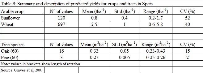
The results
are shown in the tables presented in Annexes
Table
presents the data fed into “Yield-SAFE” the biophysical model for portion of
two regions in Spain. Table gives information of the agricultural area for each
hypothetical farm and on the biophysical characteristics and the crop rotation
pattern. The data are inputs for “Yield-SAFE”. In Table is a summary and
description of predicted yields for crops and trees coming out of “Yield-SAFE”.
The last table is the outcome of the economic model, representing the
equivalent annual value of the three management systems: arable, forestry and
silvoarable system for different scenario.
The main
conclusions were
- Without grants, silvoarable systems were frequently the most profitable system at the landscape test sites.
- However, the pre-2005 grant regime altered the profitability of silvoarable systems, relative to arable and forestry systems. This was especially the case in Spain, where silvoarable systems became the least profitable system on all 19 land units.
- Under scenarios 1 and 2 of the post-2005 grant regime, support for silvoarable systems was generally predicted to be more equitable in comparison with the pre-2005 grant regime.
d) Computers-based models
Though
the aim of this review is does not include revision of sofwtares, some issues
needs to be expressed
.The complexity of the bio-economic models requires the use of software
packages (also known as computer-based models). This is also applied to
economics and biophysical models. The first forestry simulation models were
developed en the 1960s (Brown, D., 2000) (Fries 1974 cited by Graves et al,
2011)). Biophysical simulations of
agroforestry systems commenced in the 1980s (Arthur-Workshop 1984, cited by
Graves et al, 2001) and first computer models of agroforestry economics in the
1980s Arthur- Workshop 1984; Cox et al. 1988 cited by Graves et al, 2011.
Computer-based
models have a wide range, running from the use of a spreadsheet (Ms Excel) as
developed by Thomas (1991), to a dynamic model such as the developed by Justine
Namaalwa, et al (2007). In 2004, within
the Silvoarable Agroforestry for Europe (SAFE), Graves et al (2007) reviewed
the existing computer models of silvoarable economics. They describe in details
five of them POPMOD, ARBUSTRA, the Agroforestry Estate Model, WaNuLCAS, and the
Agroforestry Calculator. This is a good consulting document to have a general
idea of the state-of-the-arte in modeling in bio-economics.
V.
PRELIMINARY
CONCLUSIONS
1.- The
reviewed methodologies provides a wide range of information for decision-making
as well as on the impact of the decision.
The range of analysis is quite wide.
At the simplest extreme, it is possible to calculate the financial rate
of return of an investment in tree planting for a household, village, region,
or watershed. In the other extreme, the tools reviewed can calculate not only
financial aspects, but also economic and bio-physical aspects, leading with the
use of software to spatially location of the best alternative.
2.- The
complexity and power of the methodologies reviewed are directly correlated with
the quality of the information required. As stated in the document, data
availability is a serious limitation. The classical cost benefits analysis
required less information than the other methods. On the other extreme,
bio-economics models and software demand for high quality data and information.
3.- The
population aimed with this reviewed give high priority to income generation and
capital accumulation. Their decision is quite simple: financial profitability.
On the other side, it is known that farming decision-making impacts on the
quality of the quality of the environment and natural resources. Therefore, the
methodology for evaluation has to simple, practical and realistic. It has to
provide the demanded information but taking into account the biophysical impact
of the decision.
4.- With
the information coming out from this review the following methodology is
suggested for the practitioner level:
a) Divide the farm in sections
according to soil characteristics.
b) Select the combinations of crops and
trees for the farm.
c) Decide on the management of the
crops and trees.
d) Calculate their cost and revenues.
e) Select a proxy for the environmental benefits
of tree planting.
f) Compute the assessment using
cost/benefit analysis including the environmental benefit.
g) Select the two best alternatives (if
possible select three)
h) Run linear programming with the selected
alternatives.
i)
Analyzed
the results and select the best alternatives taking into consideration the
maximized net benefit value; the use of resources and the cost of opportunity.
5.- At the
academic level two line of research are proposed. The first one is to work in
the adjustment of the methodology proposed in number four. The second lines is
to development and organize a data base with the needed information to run more
detailed evaluation models which include biophysical data.
[1] Document
prepared within the Biodiversity management Project: Potentials and limits for
the local implementation.Technische
Universität Dresden –Facultad de Ciencias Agrarias-UNA (July, 2011). Victor Enciso
[2] World Bank Paraguay Country data profile. Available at http://data.worldbank.org/country/paraguay
[3] Ley 422/73: Artículo 42. - Todas las propiedades rurales de más de
veinte hectáreas en zonas forestales deberán mantener el veinticinco por ciento
de su área de bosques naturales. En caso de no tener este porcentaje mínimo, el
propietario deberá reforzar una superficie equivalente al cinco por ciento de
la superficie del predio.
[5] The inclusion of “production” in its name is with the
sole purpose to differentiate them from the more financial orientated coops
specialized in loan and saving schemes.
[6] Small farmers, now days known as Family Farming
include farms up to 50 hectares.
[8] In the original “Desarrollo Forestal: Opción Integrada a la Producción
Agropecuaria”
[9]
For a description of the timber business in Paraguay refer to “Timber
Investment Returns in Paraguay in
http://www.silvapar.com/publications/Frey_GE_Timber_Investment_Returns_in_Paraguay2008.pdf.
Document pending of final revision.
[11] However, there has been a
spectacular increase in the availability and quality of data from developing
countries in recent years. See http://ipl.econ.duke.edu/dthomas/dev_data/index.html for information of data in
developing countries
[12]
The simultaneous mixing in both time and space of some combination of perennial
and annual plants and/or animal production
[13] Silvoarable agroforestry is defined as the
practice of growing an arable crop between spatially zoned trees (Dupraz and Newman, 1997; Burgess
et al., 2004b, cited by Graves et al., 2007), seems the most
suitable practice for commodities farm in Paraguay.
ANEXES


No hay comentarios:
Publicar un comentario